MNIST number classification from Scratch

These notes are from Course-v4 of fastai and it differs a lot from the course-v3. In this course the have published a book call fastBook (available for free as Jupyter Notebook).

In this chapter we try to first diffrentiate nbetween 3 and 7. By cvarious techniques

1. Using pixel similarity (gives around 85% accuracy)
2. Train a Linear Model from scratch (95% acc)
   1. Optimisize this using inbuilt fastai and Pytorch classes and fns
3. Create Simple neural (non-liner = ReLU) net with 3 layers (97% acc)
4. Use cnn_learner along resnet18 as base model (9% acc)

Opening and viewing a image as tensor

im3_path = threes[0]
im3 = Image.open(im3_path)
tesnor(img) #creates img to array of pixels
df = pd.DataFrame(im3_t[4:15,4:22])
df.style.set_properties(**{'font-size':'6pt'}).background_gradient('Greys') #plots image as table of greys

• Learn to invisiona a simple base model which you think will perform reasonably well and there compare you models model with it.
• Other was is to search around for similiar problems solved by people and using those solutions with our dataset.

A list comprehension looks like this:
new_list = [f(o) for o in a_list if o>0]
This will return every element of a_list that is greater than 0, after passing it to the function f.

stack : stacks up individual tensors in a collection into a single tensor.

rank = the number of axes or dimensions of a tensor
shape = the size of each axes of a tensor

PyTorch already provides mean absolute differenc(L1 norm) root mean squared error (RMSE) (L2Norm) as loss functions. You’ll find these inside torch.nn.functional, which the PyTorch team recommends importing as F (and is available by default under that name in fastai): 

F.l1_loss(a_3.float(),mean7)
F.mse_loss(a_3,mean7).sqrt()

NumPy is the most widely used library for scientific and numeric programming in Python. It provides very similar functionality and a very similar API to that provided by PyTorch; however, it does not support using the GPU or calculating gradients, which are both critical for deep learning.
This can be jagged = can be arrays of arrays, with the innermost arrays potentially being different sizes

Pytorch Tensor restriction is that a tensor cannot use just any old type—it has to use a single basic numeric type for all components. For example, a PyTorch tensor cannot be jagged.

Crash Course on Using Tensors

1. Create a Tesnor: pass a list (or list of lists, or list of lists of lists, etc.)

   data = [[1,2,3],[4,5,6]]
   arr = array (data) #numpy
   tns = tensor(data) #pytorch tensor
   

2. Access:Tensors are 0 indexed
   Use indexes
   tns[1] is [4,5,6] #access row
   tns[:,1] is [2,5] #acces colum
   tns[1,1:3] is [5,6] #slice access 3 is excluded

3. You can use the standard operators such as +, -, *, /:
   tns+1 = [[2,3,4],[5,6,7]]

4. Tensors have a type: and wil automatically change type ex multiplies with float
   tns.type() = ‘torch.LongTensor’

Broadcasting. Pytorch will expand the tensor with the smaller rank to have the same size as the one with the larger rank. Broadcasting is an important capability that makes tensor code much easier to write.

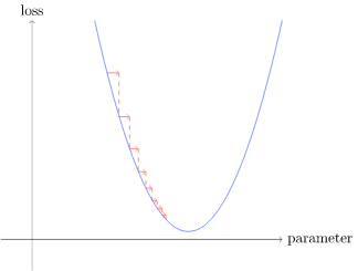
Stochastic Gradient Descent (SGD)

To minise a function we have to towards negative slope = negative gradient.
In other words, the gradients will tell us how much we have to change each weight to make our model better.
To plot a fn use (fast_ai)
plot_function(fn, x_axis, ya_xis)
to mark a point
plt.scatter(-1.5, f(-1.5), color='black');

Calculating gradient aka derivative value
xt = tensor(3.).requires_grad_()
‘_’ at end of fn indicates inplace changes ( tell PyTorch that we want to calculate gradients with respect to that variable at that value. It is essentially tagging the variable, so PyTorch will remember to keep track of how to compute gradients of the other, direct calculations on it that you will ask for.)

def f(x): return x**2
xt = tensor(3.).requires_grad_()
yt = f(xt)
yt  # = tensor(9., grad_fn=<PowBackward0>)
yt.backward() #backward propagation = calculate_gradient
xt.grad # = tensor(6.)

Tthe derivative of x**2 is 2*x, and we have x=3, so the gradients should be 2*3=6, which is what PyTorch calculated for us!

We don’t directly use the derivative adjust our weigts instead we need move slowly. The rate of moving is given by learning rate. generally it’s between 0.001 and 0.1 . Picking it is more on art than math.
The weight adjustment is given by

w -= gradient(w) * lr

Picking a low learning rate is better because if you pick too high the the loss is get worse

params.grad.data will get the grad but wont calculate it

Example to calculate Gradient descent

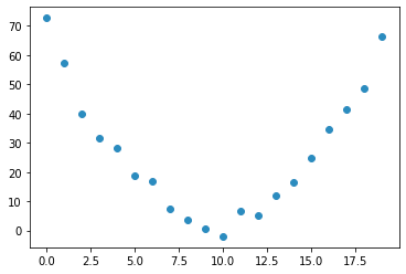
A example os a role coster going over a hill

time = torch.arange(0,20).float()
speed = torch.randn(20)*3 + 0.75*(time-9.5)**2 + 1 #some radom quadratic function
plt.scatter(time,speed);

Steps of a gradient descent:

def f(t, params):
    a,b,c = params
    return a*(t**2) + (b*t) + c #some quadratic fn our guess
    
params = torch.randn(3).requires_grad_() #random weigths
preds = f(time, params)

Initial : loss = 152.6150, random weights (got lucky)

loss.backward()
lr = 1e-5
params.data -= lr * params.grad.data
params.grad = None
preds = f(time,params)
mse(preds, speed)

1st iteration: loss = 152.3409

    
params = torch.randn(3).requires_grad_() #random weigths
lr = 1e-5

def apply_step(params, prn=True):
    preds = f(time, params)
    loss = mse(preds, speed)
    loss.backward()
    params.data -= lr * params.grad.data
    params.grad = None
    if prn: print(loss.item())
    return preds

for i in range(100): apply_step(params)

After apply step for 100 iteration: loss =125.3798828125

![aafc7974bd070abd287fb723ee1447d1.png](https://build3r.github.io/fastai//images/42a3098589994bb499bacd81204940d3.png)

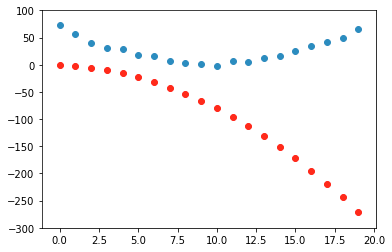
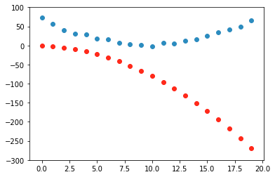
On every stem the guessed function changes as we are updating the params

### Summarizing Gradient descent:

![136f40a920e639139ada0cb589bb163d.png](https://build3r.github.io/fastai//images/2cb9308593f74007854e375869fd3d6b.png)

## MNIST Example

1.  Create training data set
    
    ```python
    train_x = torch.cat([stacked_threes, stacked_sevens]).view(-1, 28*28) #converting matrix to list
    #train_x.shape = torch.Size([12396, 784]) = 6131+6265, 28*28
    train_y = tensor([1]*len(threes) + [0]*len(sevens)).unsqueeze(1)
    #train_x.shape,train_y.shape = (torch.Size([12396, 784]), torch.Size([12396, 1]))
    dset = list(zip(train_x,train_y))
    x,y = dset[0]
    #x.shape,y =. (torch.Size([784]), tensor([1]))
    ```
    
    `view(-1,28*28)` = change a list of matrices (a rank-3 tensor) to a list of vectors (a rank-2 tensor).  
    -1 is a special parameter to view that means "make this axis as big as necessary to fit all the data"  
    `unsqueeze` = Returns a new tensor with a dimension of size one inserted at the specified position.
    
2.  Create Training Data set
    
    ```python
    valid_x = torch.cat([valid_3_tens, valid_7_tens]).view(-1, 28*28)
    valid_y = tensor([1]*len(valid_3_tens) + [0]*len(valid_7_tens)).unsqueeze(1)
    valid_dset = list(zip(valid_x,valid_y))
    ```
3.  Initialize weights
    
    ```
    def init_params(size, std=1.0):
        return (torch.randn(size)*std).requires_grad_() #random weights withe gradient required
    weights = init_params((28*28,1)) #data of 28*28, 1
    
    ```
    
    Note:  
    **Bias**: The function weights*pixels won't be flexible enough—it is always equal to 0 when the pixels are equal to 0 (i.e., its intercept is 0). You might remember from high school math that the formula for a line is y=w*x+b; we still need the b. We'll initialize it to a random number too:
    
    ```
    bias = init_params(1)
    #test one data
    (train_x[0]*weights.T).sum() + bias #.T = transpose is  because we are doing normal multiplicatin in testing not matrix mul
    # = tensor([-6.2330], grad_fn=<AddBackward0>)
    ```
4.  Do Prediction
    
    ### @ = matrix multiply
    
    ```python
    def linear1(xb): return xb@weights + bias
    preds = linear1(train_x)
    """ preds = tensor([[ -6.2330],
        [-10.6388],
        [-20.8865],
          [-15.9176],
        [ -1.6866],
        [-11.3568]], grad_fn=<AddBackward0>)"""
    ```

### Why we don't use accuracy as loss function

TLDR: small change in x ont change the prediction leading to a 0 gradient  
We have a significant technical problem here. The gradient of a function is its slope, or its steepness, which can be defined as rise over run—that is, how much the value of the function goes up or down, divided by how much we changed the input. We can write this in mathematically as: (y\_new - y\_old) / (x\_new - x\_old). This gives us a good approximation of the gradient when x\_new is very similar to x\_old, meaning that their difference is very small. But accuracy only changes at all when a prediction changes from a 3 to a 7, or vice versa. The problem is that a small change in weights from x\_old to x\_new isn't likely to cause any prediction to change, so (y\_new - y\_old) will almost always be 0. In other words, the gradient is 0 almost everywhere.

> S: In mathematical terms, accuracy is a function that is constant almost everywhere (except at the threshold, 0.5), so its derivative is nil almost everywhere (and infinity at the threshold). This then gives gradients that are 0 or infinite, which are useless for updating the model.

`torch.where(a,b,c)` == `[b[i] if a[i] else c[i] for i in range(len(a))]`

### Sigmoid fn

mnist_loss as currently defined such that it assumes that predictions are always between 0 and 1. We need to ensure, then, that this is actually the case!  
sigmoid(x) = 1/(1+e^-x)

def sigmoid(x): return 1/(1+torch.exp(-x))

Metric = what we care about  
Loss function = Similar to metric but behaves properly with gradients

5.  Defines loss function

```python
    def mnist_loss(predictions, targets):
    predictions = predictions.sigmoid()
    return torch.where(targets==1, 1-predictions, predictions).mean()

Mini Batches

We can do optimzation for single data set or the whole data set and take average in every step but it for whole dataset it take lot of time and for single it wouldn’t give much info.

So we compromise between two can calculate avg loss for few data items at a time. Which is called mini batch. Large the batch size more accurate the predictions but longer it will take to process. This also helps in parallelizingthe work in gpu.

We get better generalization if we can vary things during training. One simple and effective thing we can vary is what data items we put in each mini-batch. Rather than simply enumerating our dataset in order for every epoch, instead what we normally do is randomly shuffle it on every epoch, before we create mini-batches. PyTorch and fastai provide a class that will do the shuffling and mini-batch collation for you, called DataLoader.

When we pass a Dataset to a DataLoader we will get back many batches which are themselves tuples of tensors representing batches of independent and dependent variables

1. Gradient

    for x,y in dl:
    pred = model(x)
    loss = loss_func(pred, y)
    loss.backward() #auto gradient calculation
    parameters -= parameters.grad * lr

1. Step
   Puttling it all together weights = init_params((28*28,1)) bias = init_params(1) #create traning data loader dl = DataLoader(dset, batch_size=256) xb,yb = first(dl) #xb.shape,yb.shape = (torch.Size(\[256, 784\]), torch.Size(\[256, 1\])) #create validation dataloader valid\_dl = DataLoader(valid\_dset, batch_size=256)
   def calc_grad(xb, yb, model):
   preds = model(xb)
   loss = mnist_loss(preds, yb)
   loss.backward()
   calc_grad(batch, train_y[:4], linear1)
   #weights.grad.mean(),bias.grad = (tensor(-0.0415), tensor([-0.2826]))
   weights.grad.zero_()
   bias.grad.zero_();

loss.backward actually adds the gradients of loss to any gradients that are currently stored. So, we have to set the current gradients to 0 first.
Train:
.data: we have to tell PyTorch not to take the gradient of this step too—otherwise things will get very confusing when we try to compute the derivative at the next batch! If we assign to the data attribute of a tensor then PyTorch will not take the gradient of that step.

def train_epoch(model, lr, params):
for xb,yb in dl:
    calc_grad(xb, yb, model)
    for p in params:
        p.data -= p.grad*lr
        p.grad.zero_()

Batch Accuracy

def batch_accuracy(xb, yb):
    preds = xb.sigmoid()
    correct = (preds>0.5) == yb
    return correct.float().mean()

Validate Epoch

def validate_epoch(model):
    accs = [batch_accuracy(model(xb), yb) for xb,yb in valid_dl]
    return round(torch.stack(accs).mean().item(), 4)
``````python
validate_epoch(linear1) # 0.7175
lr = 1.
params = weights,bias
train_epoch(linear1, lr, params)
validate_epoch(linear1) #0.7313

for i in range(20):
    train_epoch(linear1, lr, params)
    print(validate_epoch(linear1), end=' ')
#0.891 0.9354 0.9491 0.9569 0.9608 0.9627 0.9637 0.9651 0.9661 0.9661 0.9671 0.9681 0.9695 0.9705 0.971 0.972 0.9735 0.9735 0.9735 0.9744 

Creating Optimizer

We now do what we did manually above with Pytorch inbuilt functionality the function linear1 = x@w + b is give by pytorch as nn.Linear

nn.Linear does the same thing as our init_params and linear together. It contains both the weights and biases in a single class.

linear_model = nn.Linear(28*28,1)

Data setup

import fastbook
fastbook.setup_book()
from fastai.vision.all import *
from fastbook import *

matplotlib.rc('image', cmap='Greys')
lr = 1e-5

path =Path( "../data/mnist_sample")#untar_data(URLs.MNIST_SAMPLE)
Path.BASE_PATH = path
threes = (path/'train'/'3').ls().sorted()
sevens = (path/'train'/'7').ls().sorted()
seven_tensors = [tensor(Image.open(o)) for o in sevens]
three_tensors = [tensor(Image.open(o)) for o in threes]
stacked_sevens = torch.stack(seven_tensors).float()/255
stacked_threes = torch.stack(three_tensors).float()/255
#validation Set
valid_3_tens = torch.stack([tensor(Image.open(o)) 
                            for o in (path/'valid'/'3').ls()])
valid_3_tens = valid_3_tens.float()/255
valid_7_tens = torch.stack([tensor(Image.open(o)) 
                            for o in (path/'valid'/'7').ls()])
valid_7_tens = valid_7_tens.float()/255

#create training data
train_x = torch.cat([stacked_threes, stacked_sevens]).view(-1, 28*28) #converting matric to list
train_y = tensor([1]*len(threes) + [0]*len(sevens)).unsqueeze(1) #We need a label for each image. Well use 1 for 3s and 0 for 7s
dset = list(zip(train_x,train_y))
dl = DataLoader(dset, batch_size=256)

#create validation data set
valid_x = torch.cat([valid_3_tens, valid_7_tens]).view(-1, 28*28)
valid_y = tensor([1]*len(valid_3_tens) + [0]*len(valid_7_tens)).unsqueeze(1)
valid_dset = list(zip(valid_x,valid_y))
valid_dl = DataLoader(valid_dset, batch_size=256)

#Loss function with sigmoid
def mnist_loss(predictions, targets):
    predictions = predictions.sigmoid()
    return torch.where(targets==1, 1-predictions, predictions).mean()

#gradient calculation
def calc_grad(xb, yb, model):
    preds = model(xb)
    loss = mnist_loss(preds, yb)
    loss.backward()

#calculate batch accuracy
def batch_accuracy(xb, yb):
    preds = xb.sigmoid()
    correct = (preds>0.5) == yb
    return correct.float().mean()
#validating one epoch
def validate_epoch(model):
    accs = [batch_accuracy(model(xb), yb) for xb,yb in valid_dl]
    return round(torch.stack(accs).mean().item(), 4)

Basic Optimizer

class BasicOptim:
    def __init__(self,params,lr): self.params,self.lr = list(params),lr

    def step(self, *args, **kwargs):
        for p in self.params: p.data -= p.grad.data * self.lr

    def zero_grad(self, *args, **kwargs):
        for p in self.params: p.grad = None
		
lr = 1e-5
opt = BasicOptim(linear_model.parameters(), lr)

Train Epoch and model

def train_epoch(model):
    for xb,yb in dl:
        calc_grad(xb, yb, model)
        opt.step()
        opt.zero_grad()
def train_model(model, epochs):
    for i in range(epochs):
        train_epoch(model)
        print(validate_epoch(model), end=' ')
train_model(linear_model, 20)

fastai provides the SGD class which, by default, does the same thing as our BasicOptim:

With inbuilt optimizer SGD

linear_model = nn.Linear(28*28,1)
opt = SGD(linear_model.parameters(), lr)
train_model(linear_model, 20)

Using Learner:

fastai also provides Learner.fit, which we can use instead of train_model. To create a Learner we first need to create a DataLoaders, by passing in our training and validation DataLoaders:

dls = DataLoaders(dl, valid_dl)
learn = Learner(dls, nn.Linear(28*28,1), opt_func=SGD,
                loss_func=mnist_loss, metrics=batch_accuracy)
learn.fit(10, lr=lr)

Adding a Nonlinearity

So we made a simple linear classifier. A linear classifier is very constrained in terms of what it can do.

def simple_net(xb): 
    res = xb@w1 + b1
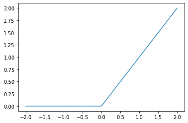
    res = res.max(tensor(0.0)) #ReLU
    res = res@w2 + b2
    return res
w1 = init_params((28*28,30))
b1 = init_params(30)
w2 = init_params((30,1))
b2 = init_params(1)

w1 and w2 are weight tensors, and b1 and b2 are bias tensors;

plot_function(F.relu)

Using Inbuilt fns

simple_net = nn.Sequential(
    nn.Linear(28*28,30),
    nn.ReLU(),
    nn.Linear(30,1)
) 
#weights and biases are auto initialised

Using Simple net

learn = Learner(dls, simple_net, opt_func=SGD,
                loss_func=mnist_loss, metrics=batch_accuracy)
learn.fit(40, 0.1)

|epoch | train_loss | valid_loss | batch_accuracy | time |—|—|—|—|–| |0| 0.313009| 0.408768| 0.507360| 00:00 |1| 0.146016| 0.232771| 0.798822| 00:00

Final Accuracy = 0.982826292514801 after 40 epochs

learn.recorder.values
[(#3) [0.31300875544548035,0.4087675213813782,0.5073601603507996],
 (#3) [0.14601589739322662,0.23277133703231812,0.7988224029541016],

the training process is recorded in learn.recorder, with the table of output stored in the values attributes

plt.plot(L(learn.recorder.values).itemgot(2)); #get batch accuracy

Visualize the weights

w,b = learn.model[0].parameters()
show_image(w[0].view(28,28))

Using full FastAi tool kit

dls = ImageDataLoaders.from_folder(path)
learn = cnn_learner(dls, resnet18, pretrained=False,
                    loss_func=F.cross_entropy, metrics=accuracy)
learn.fit_one_cycle(1, 0.1)

----------------------------------------------------------
epoch 	train_loss 	valid_loss 	accuracy 	time
0 	0.182440 	0.030915 	0.996075 	00:06

In Just 1 epoch we got accuracy of 0.996075 with power of inbuit learners and transfer learning from resnet 18

Deep learning vocabulary

Term	Meaning
ReLU	Function that returns 0 for negative numbers and doesn’t change positive numbers.
Mini-batch	A small group of inputs and labels gathered together in two arrays. A gradient descent step is updated on this batch (rather than a whole epoch).
Forward pass	Applying the model to some input and computing the predictions.
Loss	A value that represents how well (or badly) our model is doing.
Gradient	The derivative of the loss with respect to some parameter of the model.
Backward pass	Computing the gradients of the loss with respect to all model parameters.
Gradient descent	Taking a step in the directions opposite to the gradients to make the model parameters a little bit better.
Learning rate	The size of the step we take when applying SGD to update the parameters of the model.

Activations:: Numbers that are calculated (both by linear and nonlinear layers) Parameters:: Numbers that are randomly initialized, and optimized (that is, the numbers that define the model)